3  潜在结局与反事实

Note正在进行中 🚧

您正在阅读 Causal Inference in R 中文版的第一版草稿。本章节大部分已经完成，但我们可能会进行一些小的调整或文字编辑。

| 黄色的树林里分出两条路，| 可惜我不能同时涉足，| 身为旅人，我久久伫立，| 尽力眺望其中一条，| 直到它在灌木丛中转弯消失。 | — 罗伯特·弗罗斯特

2022 年，美国说唱歌手、因在 《法律与秩序：特殊受害者》 中饰演 Fin 而广为人知的 Ice-T，与人合著了 《分岔的决定：人生故事》（Split Decision: Life Stories）(Century 2022)。 在书中，Ice-T 回顾了自己从犯罪生活走向名望与成功的戏剧性历程，并将其与昔日犯罪搭档兼合著者 Spike 的命运进行对照。 两人都在洛杉矶由帮派主导的社区长大，并曾共同抢劫珠宝。 Ice-T 在一家俱乐部说唱时被人发掘，两人的人生由此分岔。 这使 Ice-T 告别犯罪生涯，开启了在音乐、电影和电视领域的成功事业。 与此同时，Spike 在一次珠宝抢劫中被捕，并入狱三年。 此后他继续犯罪，最终因一次失败的抢劫被判处 35 年至终身监禁。 该书的宣传文案写道：“两个生活截然不同的人揭示，如果当初作出不同选择，他们的人生道路很可能会彼此对调。”

这一引人入胜的前提意味着，我们正在观察反事实：两段人生原本沿着相同轨迹前进，直到一个决定（再实施一次抢劫，还是追求音乐事业）使它们分岔，一段人生通向监狱，另一段则通向成功与名望。 本书开篇先说明 Ice-T 与朋友 Spike 在人生分岔前的种种相似之处（例如，两人都在洛杉矶的社区长大，都与帮派有关，并曾合作策划一系列珠宝抢劫）。 随后发生了变化：Ice-T 放弃犯罪生活，而 Spike 作出了相反的决定。 此后，Ice-T 收获名望与财富，Spike 则被判处 35 年至终身监禁。 这本书尝试对两个人进行一项小型研究：他们在某个事件发生前相同，事件发生后却变得不同。 Spike 的结局可作为 Ice-T 结局的反事实。

flowchart LR
A{Ice-T} --> |observed| B(Abandons criminal life)
A -.-> |missing counterfactual| C(Does one more heist)
C -.-> D[35 years in prison]
B --> E[Fame & Fortune]

classDef grey fill:#ddd
class D,C grey

flowchart LR
A{Spike} -.-> |missing counterfactual| B(Abandons criminal life)
A --> |observed| C(Does one more heist)
C --> D[35 years in prison]
B -.-> E[Fame & Fortune]
classDef grey fill:#ddd
class E,B grey

Table 3.1: Ice-T 与 Spike 的因果图。 对于这两个人，我们各自只能观察到一个结局。 他们的回忆录暗示，二人都可作为彼此良好的反事实。 如果 Ice-T 继续抢劫，他最终会入狱吗？ 如果 Spike 停止抢劫，他会获得名望和财富吗？

我们不知道，如果 Ice-T 继续与 Spike 合伙抢劫，他会经历什么。 我们也不知道，如果 Spike 像 Ice-T 一样远离犯罪，他会有怎样的人生。 我们生活在唯一的事实世界中：Ice-T 离开了犯罪生活，而 Spike 没有。 不过，我们可以看出，二人如何能够彼此代理那些反事实结局。 因果推断技术也以非常相似的方式，尝试使用观察数据来模拟反事实。 即使随机试验也只能存在于一个事实世界中，因此我们比较具有不同暴露的相似组之间的平均效应。

尽管如此，我们马上就能看到几个问题，凸显出作出此类推断的困难。 首先，虽然本书暗示两人在作出使命运分岔的决定之前十分相似，但我们仍可以推测他们可能有哪些不同。 再实施一次抢劫会让 Ice-T 入狱吗？ 在这个方向上，较容易将 Spike 视为良好的反事实。 那么反过来呢：如果 Spike 退出犯罪生活，他会成为著名的音乐家和演员吗？ Ice-T 决定告别犯罪生活，但这并不是他成功的唯一因素：他拥有足以成就事业的音乐才华。 Spike 是否也拥有 Ice-T 的音乐才华？ 我们能否断定，如果 Spike 作出同样的选择，他的人生就会与 Ice-T 完全相同？ 如果想真正估计 Ice-T 决定离开犯罪生活对其未来结局的因果效应，就需要同时观察他作出这一决定与不作出这一决定时最终会走上怎样的道路。 同样，Spike 可能在一些难以测量的方面不同于 Ice-T，因此他对 Ice-T 反事实的代理能力可能不如初看时那么好。 我们通常不会只依赖一个人，而是依赖许多人。 我们可以开展一项实验，将许多人随机分配为离开或不离开犯罪生活，并观察这对其平均结局有何影响（当然，这种随机试验存在一些伦理问题，而这也正是 Ice-T 和 Spike 这样的观察数据令人感兴趣的原因）。 无论如何，我们必须借助统计技术，利用观察数据构建这些不可观察的反事实。

3.1 潜在结局

事实结局和反事实结局是潜在结局的两种实现。 在某个原因发生之前，潜在结局是根据个体所接受的暴露可能发生的所有结果。 假设我们关注的原因发生在 20 世纪 80 年代的某个特定时刻，当时一个人决定停止或继续实施珠宝抢劫。 我们关注的结局是该个体是否入狱。

假设某项暴露有两个水平：

• 若继续实施珠宝抢劫，则 \(X=continue\)

• 若停止实施珠宝抢劫，则 \(X=quit\)

在这一情景下，存在两个潜在结局：

• \(Y(continue)\)，即 \(X=continue\) 时的潜在结局

• \(Y(quit)\)，即 \(X=quit\) 时的潜在结局

这些潜在结局中只有一个会实现，即与实际发生的暴露相对应的事实结局。 因此，对每个个体只能观察到一个潜在结局。 这些暴露是在某个特定时间点定义的（在本例中，是 20 世纪 80 年代 Ice-T 刚被发掘前后的某个时刻），所以任何个体只能经历其中一种暴露。 对于二元暴露，这意味着一个潜在结局是可观察的，另一个则是缺失的。事实上，早期因果推断方法常被表述为缺失数据问题；我们需要对缺失的反事实，即与未发生暴露相对应的潜在结局值，作出某些假设。

我们关注的因果效应通常是潜在结局之间的某种差异，例如 \(Y(continue) - Y(quit)\)（比如，继续抢劫与停止抢劫相比，次年入狱概率的差异）。 对于 Ice-T 和 Spike，我们关注的是他们各自的个体因果效应：

• \(Y_{Ice-T}(continue) - Y_{Ice-T}(quit)\)
• \(Y_{Spike}(continue) - Y_{Spike}(quit)\)

这里缺少 \(Y_{Ice-T}(continue)\) 和 \(Y_{Spike}(quit)\)，因此无法计算这些值。 在实践中，我们需要用观察数据代理缺失的潜在结局，并通常在特定人群中对其取平均值。 但要做到这一点，不能只是对一堆观察数据随意运用统计方法；我们需要满足某些因果假设，使观察数据能够具有潜在结局的含义，并使相应分析能够解释为因果效应。

Note作为潜在结局的反事实

本书在很大程度上交替使用”潜在结局”和”反事实”这两个术语，但严格来说，它们的含义并不完全相同。 反事实是潜在结局的一种，指未实现、因而不可观察的潜在结局。 反事实的定义取决于实际发生的暴露。 潜在结局则不依赖于观察到的暴露，而且常常在暴露发生前就已得到良好定义。 尽管如此，我们通常处理的是暴露发生后的数据，因此会有一个已经实现的潜在结局，以及至少一个与事实相反的潜在结局。 有些坚定的拥护者坚持只使用其中一个术语，但我们认为两者都有用。

让我们考虑另一个例子：冰淇淋对幸福感的影响。

3.1.1 巧克力冰淇淋比香草冰淇淋更让人快乐吗？

假设存在一个范围为 1–10 的幸福感指数。 我们希望评估，与香草冰淇淋相比，食用巧克力冰淇淋是否会提高幸福感。 现有 10 名个体，每人都有两个潜在结局。 一个是食用巧克力冰淇淋时的幸福感（在下面的代码中定义为 y_chocolate），另一个是食用香草冰淇淋时的幸福感（y_vanilla）。 对于每名个体，我们可以将食用巧克力冰淇淋（相对于香草冰淇淋）对幸福感的真实个体因果效应定义为二者之差（Table 3.2）。

data <- tibble(
  id = 1:10,
  y_chocolate = c(4, 4, 6, 5, 6, 5, 6, 7, 5, 6),
  y_vanilla = c(1, 3, 4, 5, 5, 6, 8, 6, 3, 5)
)

data <- data |>
  mutate(causal_effect = y_chocolate - y_vanilla)

library(gt)
data |>
  gt() |>
  cols_label(
    id = "ID",
    y_chocolate = md("$$Y_{\\text{id}}(\\text{chocolate})$$"),
    y_vanilla = md("$$Y_{\\text{id}}(\\text{vanilla})$$"),
    causal_effect = md(
      "$$Y_{\\text{id}}(\\text{chocolate}) - Y_{\\text{id}}(\\text{vanilla})$$"
    )
  ) |>
  fmt_markdown(
    columns = c(y_chocolate, y_vanilla, causal_effect)
  ) |>
  tab_header(
    title = md("**Potential Outcomes and Causal Effect**")
  ) |>
  tab_spanner(
    label = "Potential Outcomes",
    columns = c(y_chocolate, y_vanilla)
  ) |>
  tab_spanner(
    label = "Causal Effect",
    columns = causal_effect
  )

Potential Outcomes and Causal Effect
ID	Potential Outcomes		Causal Effect
	\[Y_{\text{id}}(\text{chocolate})\]	\[Y_{\text{id}}(\text{vanilla})\]	\[Y_{\text{id}}(\text{chocolate}) - Y_{\text{id}}(\text{vanilla})\]
1	4	1	3
2	4	3	1
3	6	4	2
4	5	5	0
5	6	5	1
6	5	6	-1
7	6	8	-2
8	7	6	1
9	5	3	2
10	6	5	1

Table 3.2: 潜在结局模拟：食用巧克力冰淇淋（相对于香草冰淇淋）对幸福感的因果效应。在该模拟中，每名个体在每种暴露下的结局均已知。由于已知每个潜在结局，我们可以计算食用巧克力冰淇淋相对于香草冰淇淋对幸福感的个体因果效应。

例如，查看 Table 3.2， 食用巧克力冰淇淋（相对于香草冰淇淋）对第 4 名个体的因果效应为 0，而对第 9 名个体的因果效应为 2。

食用巧克力冰淇淋后的平均潜在幸福感为 5.4，食用香草冰淇淋后的平均潜在幸福感为 4.6。 在本研究的 10 名个体中，食用巧克力冰淇淋（相对于香草冰淇淋）的平均处理效应为 5.4 - 4.6 = 0.8。

data |>
  summarize(
    avg_chocolate = mean(y_chocolate),
    avg_vanilla = mean(y_vanilla),
    avg_causal_effect = mean(causal_effect)
  )

# A tibble: 1 × 3
  avg_chocolate avg_vanilla avg_causal_effect
          <dbl>       <dbl>             <dbl>
1           5.4         4.6               0.8

现实中，我们无法在任一时刻同时观察到两个潜在结局；研究进行时，每名个体只能食用一种口味的冰淇淋¹。 假设我们随机给每名参与者分配其中一种口味。 此时，我们观察到的内容如 Table 3.3 所示。 我们只知道一个潜在结局（与参与者实际接受的暴露相关的结局）。 另一个潜在结局未知，因此个体因果效应也未知。

## 下面会执行随机操作，因此设置随机种子，
## 以确保每次运行代码时
## 都能观察到相同的结果
set.seed(11)
data_observed <- data |>
  mutate(
    # 将暴露改为随机生成，其来源为
    # 成为任一组的概率均为 0.5 的
    # 二项分布
    exposure = if_else(
      rbinom(n(), 1, 0.5) == 1,
      "chocolate",
      "vanilla"
    ),
    observed_outcome = case_when(
      exposure == "chocolate" ~ y_chocolate,
      exposure == "vanilla" ~ y_vanilla
    )
  )

avg_chocolate <- data_observed |>
  filter(exposure == "chocolate") |>
  pull(observed_outcome) |>
  mean()

avg_vanilla <- data_observed |>
  filter(exposure == "vanilla") |>
  pull(observed_outcome) |>
  mean()

data_observed |>
  mutate(
    y_chocolate = if_else(exposure == "chocolate", y_chocolate, NA),
    y_vanilla = if_else(exposure == "vanilla", y_vanilla, NA),
    causal_effect = NA_real_
  ) |>
  select(-observed_outcome, -exposure) |>
  gt() |>
  cols_label(
    id = "ID",
    y_chocolate = md("$$Y_{\\text{id}}(\\text{chocolate})$$"),
    y_vanilla = md("$$Y_{\\text{id}}(\\text{vanilla})$$"),
    causal_effect = md(
      "$$Y_{\\text{id}}(\\text{chocolate}) - Y_{\\text{id}}(\\text{vanilla})$$"
    )
  ) |>
  fmt_markdown(columns = c(y_chocolate, y_vanilla, causal_effect)) |>
  sub_missing(
    columns = c(y_chocolate, y_vanilla, causal_effect),
    missing_text = md("---") # Format missing values as blank
  ) |>
  tab_header(
    title = md("**Potential Outcomes and Hidden Causal Effect**")
  ) |>
  tab_spanner(
    label = "Potential Outcomes",
    columns = c(y_chocolate, y_vanilla)
  ) |>
  tab_spanner(
    label = "Causal Effect",
    columns = causal_effect
  )

Potential Outcomes and Hidden Causal Effect
ID	Potential Outcomes		Causal Effect
	\[Y_{\text{id}}(\text{chocolate})\]	\[Y_{\text{id}}(\text{vanilla})\]	\[Y_{\text{id}}(\text{chocolate}) - Y_{\text{id}}(\text{vanilla})\]
1	—	1	—
2	—	3	—
3	6	—	—
4	—	5	—
5	—	5	—
6	5	—	—
7	—	8	—
8	—	6	—
9	5	—	—
10	—	5	—

Table 3.3: 潜在结局模拟：观察到的暴露对应于我们唯一已知的潜在结局。由于不知道缺失的潜在结局，因此无法计算个体因果效应。我们需要使用观察到的暴露和结局，估计食用巧克力冰淇淋（相对于香草冰淇淋）对幸福感的影响。遗憾的是，我们无法在个体水平上完成这一估计。

现在，食用巧克力冰淇淋者的观察平均结局为 5.3，食用香草冰淇淋者则为 4.7。 尽管现在缺失反事实结局，这些数值仍接近真实平均值。 估计的平均因果效应为 5.3 - 4.7 = 0.6。 由于样本量较小，结果略有偏差；随着样本量增加，我们会得到更精确的答案。

data_observed |>
  group_by(exposure) |>
  summarise(avg_outcome = mean(observed_outcome))

# A tibble: 2 × 2
  exposure  avg_outcome
  <chr>           <dbl>
1 chocolate        5.33
2 vanilla          4.71

既然已经无法计算真实因果效应，为什么这种做法仍然有效？ 事实证明，随机化具有使观察数据满足因果假设所需的性质。 由于满足这些假设，我们可以用观察平均值代理两个潜在结局的平均值。

下面看看其中的原因，以及这些假设被违反时会发生什么。

3.2 因果假设

本书将讨论许多方法。 每种方法都伴随着无法验证的假设；要将结果解释为因果关系，就必须依赖这些假设。 这些假设只有一个目标：使我们能够用观察数据表示不可观察的反事实。 要做到这一点，需要满足哪些条件？

Note同类相比

因果推断所需的大多数假设，都是为了进行”同类相比”：我们希望比较相似的个体，使其能够合理地代理彼此的反事实。

“同类相比”（apples-to-apples）源自”拿苹果和橙子比较”（comparing apples to oranges）这一说法，后者意指比较两个不可比的事物。

这只是一种说法。 世界各地还有许多不同版本。 下面是一些人们不应尝试相互比较的事物：

• 奶酪和粉笔（英国英语）
• 苹果和梨（德语）
• 马铃薯和甘薯（拉丁美洲西班牙语）
• 祖母和蟾蜍（塞尔维亚语）
• 马和驴（印地语）

在本书大约前四分之三的内容中，我们将处理所谓的无混杂性方法。 这些方法都作出²三个假设：可交换性、正值性和一致性。 目前我们将聚焦于这三个假设；但其他方法，如工具变量分析 (?sec-iv-friends) 和双重差分法 (?sec-did) ，会作出其他因果假设。了解一种方法的假设对正确使用它至关重要；同时，也值得考虑其他方法的假设对于你试图解决的问题是否更站得住脚。

这些假设有时称为可识别性条件，因为只有它们成立时才能识别因果估计。 类似地，你有时会看到人们讨论某个给定因果效应是否”可识别”。

3.2.1 可交换性

可交换性假设是逆概率加权、回归调整等无混杂性方法的标志。 在此，我们假设各暴露组平均具有相同的潜在结局。 因此，被分配巧克力冰淇淋的组，其巧克力口味下的平均幸福感潜在结局，与香草组在假如被分配巧克力口味时的潜在结局相同。 在数学上，可交换性写作 \(Y(x) \perp\!\!\!\perp X\)。 暴露状态独立于潜在结局；例如，与处于香草组相比，处于巧克力组并不会改变你的潜在结局 y(chocolate)。 当这一假设成立时，我们可以把香草组视为巧克力组 y(vanilla) 的代理，反之亦然，如 Figure 3.1 所示。

plot_data <- data_observed |>
  select(starts_with("y"), exposure) |>
  mutate(id = row_number()) |>
  prepare_plot_data(
    pivot_prefix = "y_",
    potential_outcome_transform = \(x) paste0("potential outcome: y(", x, ")"),
    transform_exposure = \(exp) {
      if_else(
        exp == "vanilla",
        "actually ate vanilla",
        "actually ate chocolate"
      )
    },
    id_assignment = FALSE
  )

# Compute group averages and add label text
avg_labels <- compute_avg_labels(
  plot_data,
  c("potential_outcome", "exposure", "observed")
) |>
  mutate(
    exposure_lbl = str_replace_all(exposure, "actually ate ", ""),
    po_lbl = str_replace_all(potential_outcome, "potential outcome: ", ""),
    label = glue("Avg {po_lbl}\n({exposure_lbl} group, {observed})") |>
      str_wrap(19)
  )

# Prepare an annotation for ID 3
id_annotation <- plot_data |>
  filter(id == 3) |>
  mutate(
    label = glue("Potential outcomes\nfor ID 3 ({observed})") |> str_wrap(15)
  )

# Exchangeability annotation between group averages
exchangeability_annotation <- tibble(
  x = 5.43,
  xend = 5.33,
  y = 1,
  yend = 0.5,
  potential_outcome = "potential outcome: y(chocolate)",
  label = str_wrap(
    "For exchangeability to hold, these\ngroup averages should be similar",
    19
  )
)

ggplot(plot_data, aes(happiness, y_id, color = observed, shape = observed)) +
  geom_point(aes(fill = observed), size = 3, alpha = 0.8) +
  add_avg_layers(
    avg_labels,
    observed_col = ggokabeito::palette_okabe_ito(1),
    unobserved_col = ggokabeito::palette_okabe_ito(2)
  ) +
  geom_curve(
    data = id_annotation,
    mapping = aes(
      x = happiness + 2.5,
      xend = happiness + 0.5,
      y = y_id + 2,
      yend = y_id
    ),
    curvature = -0.2,
    arrow = arrow(length = unit(0.02, "npc")),
    inherit.aes = FALSE,
    color = "grey40"
  ) +
  geom_label(
    data = id_annotation,
    mapping = aes(x = happiness + 2, y = y_id + 1.5, label = label),
    hjust = 0,
    inherit.aes = FALSE,
    color = "grey40",
    size = 3.75,
    linewidth = NA
  ) +
  geom_curve(
    data = exchangeability_annotation,
    mapping = aes(x = x + 0.5, xend = xend + 0.2, y = y + 0.5, yend = yend),
    curvature = 0.1,
    arrow = arrow(length = unit(0.02, "npc")),
    inherit.aes = FALSE,
    color = "grey40"
  ) +
  geom_label(
    data = exchangeability_annotation,
    mapping = aes(x = x + 0.05, y = y, label = label),
    inherit.aes = FALSE,
    hjust = "left",
    nudge_x = 0.5,
    color = "grey40",
    size = 4,
    linewidth = NA
  ) +
  facet_wrap(~potential_outcome) +
  scale_y_continuous(
    breaks = c(unique(plot_data$y_id), min(plot_data$y_id) - 1),
    labels = c(unique(plot_data$id), expression(bold("Avg")))
  ) +
  scale_shape_manual(
    name = NULL,
    values = c(19, 21)
  ) +
  scale_fill_manual(
    name = NULL,
    values = c(
      "observed" = ggokabeito::palette_okabe_ito(1),
      "unobserved" = "white"
    )
  ) +
  scale_color_manual(
    name = NULL,
    values = c(
      "observed" = ggokabeito::palette_okabe_ito(1),
      "unobserved" = ggokabeito::palette_okabe_ito(2)
    )
  ) +
  scale_x_continuous(
    breaks = seq(0, 12, by = 2.5),
    limits = c(NA, 12)
  ) +
  po_theme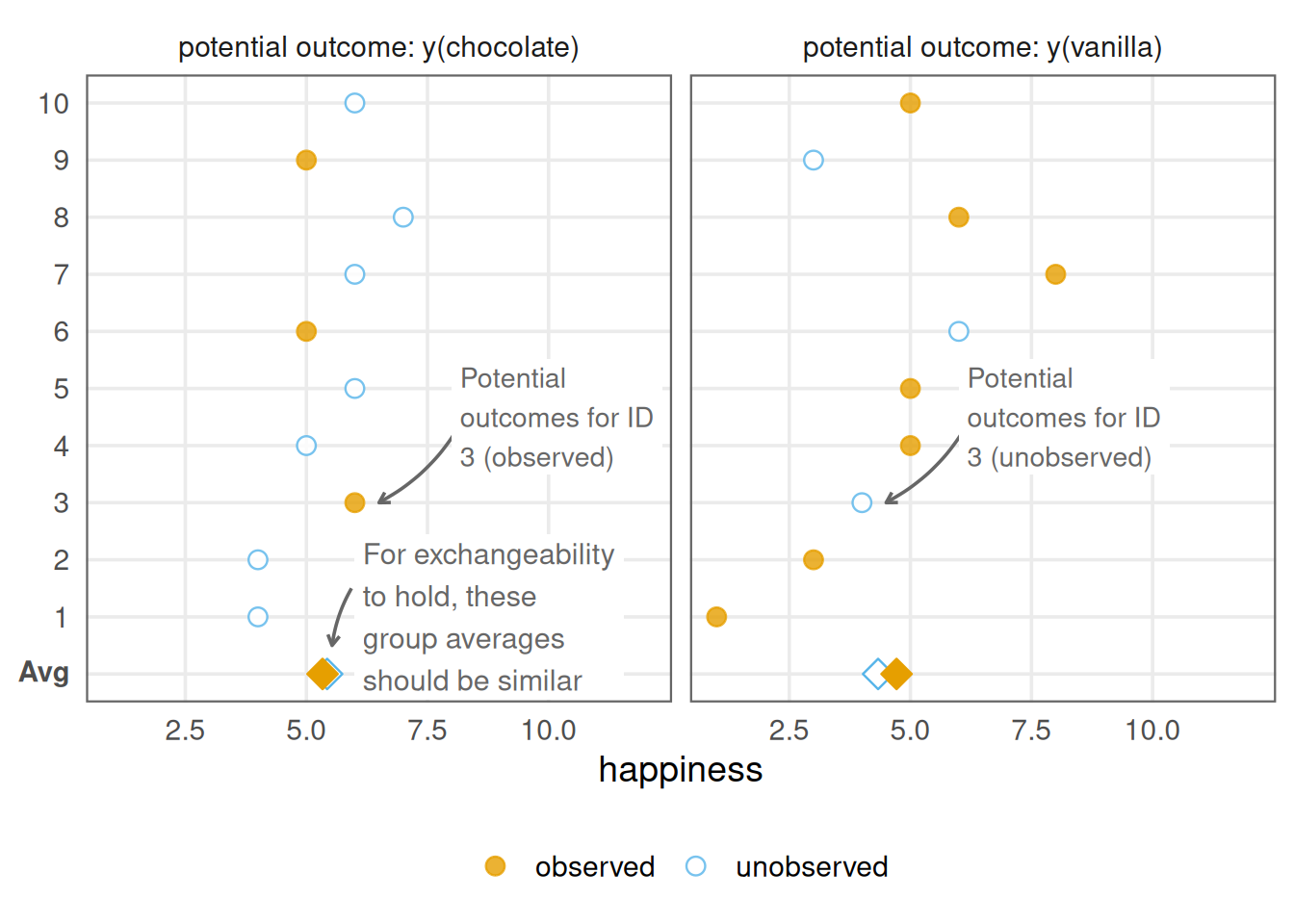

Figure 3.1: 按观察暴露组划分的平均潜在结局。在可交换性成立时，暴露组别与潜在结局无关。若香草组接受巧克力口味，其平均潜在结局会与巧克力组大致相同，反之亦然。可交换性使我们能够将每组作为另一组的反事实。

可交换性有时称为”无混杂”或”无混杂性”假设。 它有时也称为”可忽略性”。

像前面随机分配冰淇淋口味那样对暴露实施随机化时，可交换性在极限意义下得到保证。 从随机化过程的角度考虑可交换性，就能理解这个名称的由来。 假设我们混淆了谁获得哪种口味的标签，误把巧克力分给”香草”组，又把香草分给”巧克力”组。 由于口味分配独立于潜在结局，这种混淆并不重要。 我们通过反转分配交换了两组，但仍然可以检测到正确的因果效应 ³。

set.seed(11)

mix_up <- function(flavor) {
  if_else(flavor == "chocolate", "vanilla", "chocolate")
}

data_observed <- data |>
  mutate(
    exposure = if_else(
      rbinom(n(), 1, 0.5) == 1,
      "chocolate",
      "vanilla"
    ),
    exposure = mix_up(exposure),
    observed_outcome = case_when(
      exposure == "chocolate" ~ y_chocolate,
      exposure == "vanilla" ~ y_vanilla
    )
  )

data_observed |>
  group_by(exposure) |>
  summarise(avg_outcome = mean(observed_outcome))

# A tibble: 2 × 2
  exposure  avg_outcome
  <chr>           <dbl>
1 chocolate        5.43
2 vanilla          4.33

那么，违反可交换性意味着什么？ 假设我们改为允许每名参与者自行选择冰淇淋口味。 参与者有 80% 的概率选择最能让自己快乐的口味—也就是其偏好口味。

set.seed(113)
data_observed_exch <- data |>
  mutate(
    prefer_chocolate = y_chocolate > y_vanilla,
    exposure = case_when(
      # people who like chocolate more chose that 80% of the time
      prefer_chocolate ~ if_else(
        rbinom(n(), 1, 0.8) == 1,
        "chocolate",
        "vanilla"
      ),
      # people who like vanilla more chose that 80% of the time
      !prefer_chocolate ~ if_else(
        rbinom(n(), 1, 0.8) == 1,
        "vanilla",
        "chocolate"
      )
    ),
    observed_outcome = case_when(
      exposure == "chocolate" ~ y_chocolate,
      exposure == "vanilla" ~ y_vanilla
    )
  )

现在，看起来反而是香草口味更让人快乐！

data_observed_exch |>
  group_by(exposure) |>
  summarise(avg_outcome = mean(observed_outcome))

# A tibble: 2 × 2
  exposure  avg_outcome
  <chr>           <dbl>
1 chocolate        5.29
2 vanilla          5.67

为什么会这样？ 我们将在 Chapter 4 及后续内容中更深入地探讨这个问题；但从假设角度看，可交换性已不再成立。 两个暴露组的平均潜在结局不再相同。 两组的 y(chocolate) 平均值仍然相当接近，但 y(vanilla) 在组间差异很大。 香草组不再能很好地代理巧克力组的潜在结局，因而产生了有偏结果。 这里实际看到的是 y(flavor, preference) 的潜在结局。 这始终是事实，因为有些个体的个体因果效应不为 0。 发生变化的是，潜在结局不再独立于一个人获得的 flavor：其偏好同时影响口味选择和潜在结局。 如 Figure 3.2 所示，各组不再可交换；它们的 y(vanilla) 平均潜在结局并不相同。

data_observed_exch |>
  select(starts_with("y"), exposure) |>
  pivot_longer(
    starts_with("y"),
    names_prefix = "y_",
    names_to = "potential_outcome",
    values_to = "happiness"
  ) |>
  mutate(
    observed = if_else(exposure == potential_outcome, "observed", "unobserved"),
    potential_outcome = paste0("potential outcome: y(", potential_outcome, ")"),
    exposure = if_else(
      exposure == "vanilla",
      "actually ate\nvanilla",
      "actually ate\nchocolate"
    )
  ) |>
  ggplot(aes(
    happiness,
    exposure,
    color = observed,
    fill = observed,
    shape = observed
  )) +
  stat_summary(
    fun = "mean",
    size = 3.5,
    geom = "point",
    shape = 23,
    position = position_nudge(y = 0.033)
  ) +
  stat_summary(
    fun = "mean",
    geom = "text",
    aes(label = round(after_stat(x), 1)),
    vjust = 1.8,
    show.legend = FALSE
  ) +
  facet_wrap(~potential_outcome) +
  theme(
    panel.grid.major.y = element_blank(),
    panel.border = element_rect(color = "grey40", fill = NA, linewidth = 0.8),
    axis.title.y = element_blank()
  ) +
  labs(
    y = "actual exposure",
    color = NULL,
    shape = NULL,
    fill = NULL
  ) +
  coord_cartesian(clip = "off") +
  scale_shape_manual(values = c(19, 21)) +
  scale_fill_manual(
    values = c(
      observed = ggokabeito::palette_okabe_ito(1),
      unobserved = "white"
    )
  ) +
  scale_x_continuous(breaks = seq(0, 12, by = 2.5), limits = c(-2, 12))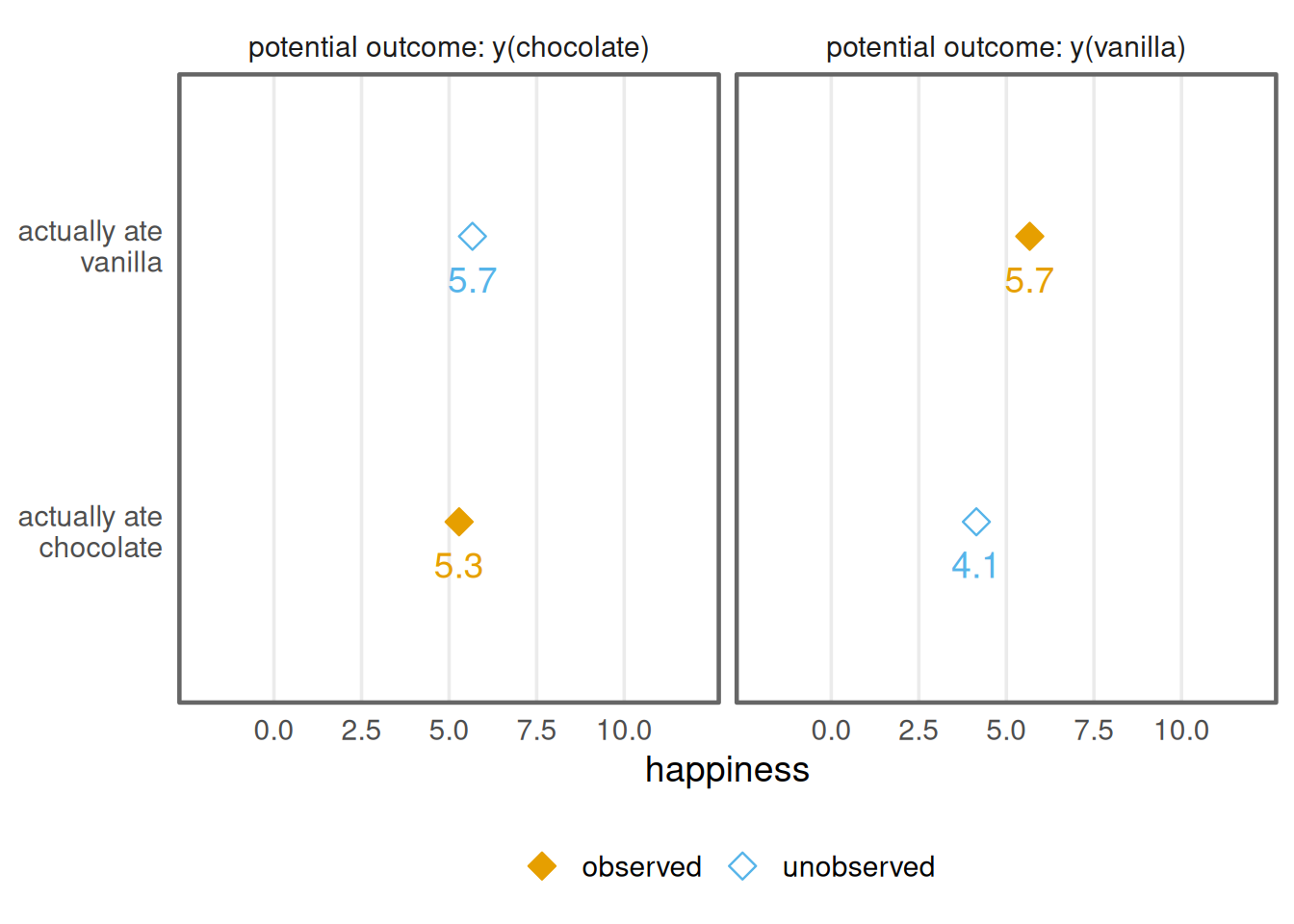

Figure 3.2: 存在混杂时，按观察暴露组划分的平均潜在结局。由于口味分配不再独立于潜在结局，各组不再具有可交换性。

违反可交换性时该怎么办？ 本书将用大量篇幅讨论这个问题。 解决方案的核心是，有时我们仍能在另一个变量的各水平内实现可交换性。 这称为条件可交换性：\(Y(x) \perp\!\!\!\perp X \mid Z\)。 在本例中，我们需要在 prefer_chocolate 的各水平内实现可交换性。

data_observed_exch |>
  mutate(
    prefer_chocolate = if_else(
      prefer_chocolate,
      "prefers\nchocolate",
      "prefers\nvanilla"
    )
  ) |>
  pivot_longer(
    starts_with("y"),
    names_prefix = "y_",
    names_to = "potential_outcome",
    values_to = "happiness"
  ) |>
  mutate(
    observed = if_else(exposure == potential_outcome, "observed", "unobserved"),
    potential_outcome = paste0("potential outcome: y(", potential_outcome, ")"),
    exposure = if_else(
      exposure == "vanilla",
      "actually ate\nvanilla",
      "actually ate\nchocolate"
    )
  ) |>

  ggplot(aes(
    happiness,
    exposure,
    color = observed,
    fill = observed,
    shape = observed
  )) +
  stat_summary(
    fun = "mean",
    size = 3.5,
    geom = "point",
    shape = 23,
    position = position_nudge(y = 0.033)
  ) +
  stat_summary(
    fun = "mean",
    geom = "text",
    aes(label = round(after_stat(x), 1)),
    vjust = 1.8,
    show.legend = FALSE
  ) +
  facet_grid(prefer_chocolate ~ potential_outcome) +
  theme(
    panel.grid.major.y = element_blank(),
    panel.border = element_rect(color = "grey40", fill = NA, linewidth = 0.8),
    axis.title.y = element_blank()
  ) +
  labs(
    y = "actual exposure",
    color = NULL,
    shape = NULL,
    fill = NULL
  ) +
  coord_cartesian(clip = "off") +
  scale_shape_manual(values = c(19, 21)) +
  scale_fill_manual(
    values = c(
      observed = ggokabeito::palette_okabe_ito(1),
      unobserved = "white"
    )
  ) +
  scale_x_continuous(breaks = seq(0, 12, by = 2.5), limits = c(-2, 12))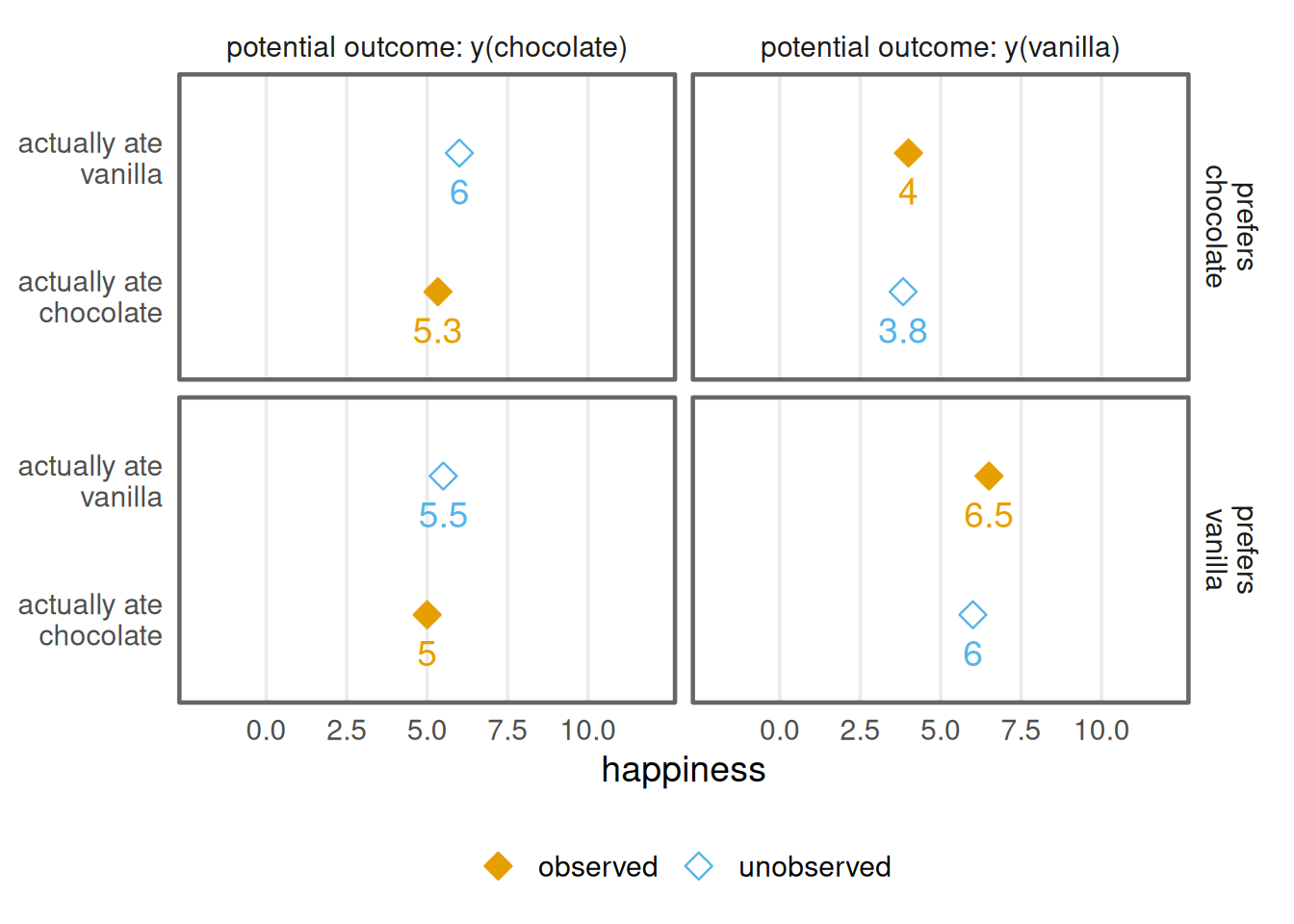

Figure 3.3: 存在混杂时，按观察暴露组划分的平均潜在结局。我们仍可以在混杂因素的各水平内实现条件可交换性。这里也开始显现样本量的局限：在更大样本下本应成立的潜在结局关系开始失效。

在 Figure 3.3 中，我们已经开始遭遇维数灾难：样本量太小，暴露与偏好各组合下的观测值非常少。 随着样本量增加，可交换性会有所改善；但若没有良好的统计模型，这很快就会变得困难。

3.2.2 正值性

正值性假设指出，每名个体接受每个暴露水平的概率都不为零。 在数学上，这意味着对所有 \(x\)，都有 \(P(X = x) > 0\)。 换言之，我们假设不存在某些人绝不可能接受一个或多个暴露水平。 之所以需要这一假设，是因为它定义了给定暴露水平下的潜在结局。 如果某人在任何情况下都绝不会暴露于巧克力，那么该个体的潜在结局 y(chocolate) 就没有定义。 我们无法利用此人提供关于该潜在结局的信息。 在随机试验中，暴露概率由设计确定，因而是已知的。 在冰淇淋示例中，每个人的概率都相同：接受巧克力口味的概率为 50%，接受香草口味的概率也为 50%。 这些可能性为两组定义了两个潜在结局。

正值性有时称为概率性假设。

违反正值性有两种形式：随机性违反和结构性违反。 随机性违反是偶然发生的情形，即给定暴露水平下没有任何观测值。 在参与者有 80% 的概率选择最让自己快乐的冰淇淋这一示例中，由于样本量较小，完全可能出现某类人只选择巧克力的情况。 显然，只有在拥有香草口味的观测值时，我们才能计算香草相对于巧克力的效应。

正值性的一个细微之处在于，它需要在实现可交换性所需的所有协变量水平内成立：对所有 \(x\) 和 \(z\)，都有 \(P(X = x \mid Z = z) > 0\)。 即使口味总体上存在变异，我们也需要在 prefer_chocolate 的各水平内存在变异。 这一条件也可能偶然失效。

set.seed(1)
data_observed_pos <- data |>
  mutate(
    prefer_chocolate = y_chocolate > y_vanilla,
    exposure = case_when(
      prefer_chocolate ~ if_else(
        rbinom(n(), 1, 0.8) == 1,
        "chocolate",
        "vanilla"
      ),
      !prefer_chocolate ~ if_else(
        rbinom(n(), 1, 0.8) == 1,
        "vanilla",
        "chocolate"
      )
    ),
    observed_outcome = case_when(
      exposure == "chocolate" ~ y_chocolate,
      exposure == "vanilla" ~ y_vanilla
    )
  )

data_observed_pos |>
  count(prefer_chocolate, exposure) |>
  complete(
    prefer_chocolate,
    exposure = c("chocolate", "vanilla"),
    fill = list(n = 0)
  )

# A tibble: 4 × 3
  prefer_chocolate exposure      n
  <lgl>            <chr>     <int>
1 FALSE            chocolate     0
2 FALSE            vanilla       3
3 TRUE             chocolate     7
4 TRUE             vanilla       0

结构性正值性违反是指，按照定义，某个体不可能接受至少一个暴露水平。 假设部分参与者对香草过敏。 即使在随机化情境中，这些参与者也不能食用香草口味。 在本例中，假设任何对香草过敏但被分配香草口味的人都会改为巧克力口味。

set.seed(11)
data_observed_struc <- data |>
  mutate(
    exposure = if_else(
      rbinom(n(), 1, 0.5) == 1,
      "chocolate",
      "vanilla"
    )
  )

set.seed(1)
data_observed_struc <- data_observed_struc |>
  mutate(
    # 30% chance of allergy
    allergy = rbinom(n(), 1, 0.3) == 1,
    # in which case `y_vanilla` is impossible
    exposure = if_else(allergy, "chocolate", exposure),
    y_vanilla = if_else(allergy, NA, y_vanilla),
    observed_outcome = case_when(
      # those with allergies always take chocolate
      allergy ~ y_chocolate,
      exposure == "chocolate" ~ y_chocolate,
      exposure == "vanilla" ~ y_vanilla
    )
  )

现在，我们的估计出现了相当大的偏差。

data_observed_struc |>
  group_by(exposure) |>
  summarise(avg_outcome = mean(observed_outcome))

# A tibble: 2 × 2
  exposure  avg_outcome
  <chr>           <dbl>
1 chocolate         5.4
2 vanilla           4  

对于香草过敏者，y_vanilla 没有定义，如 Figure 3.4 所示。

plot_data <- data_observed_struc |>
  mutate(is_missing_y_vanilla = is.na(y_vanilla)) |>
  select(id, starts_with("y"), exposure, is_missing_y_vanilla) |>
  prepare_plot_data(
    pivot_prefix = "y_",
    potential_outcome_transform = \(x) paste0("y(", x, ")"),
    transform_exposure = \(exp) {
      if_else(
        exp == "vanilla",
        "actually ate vanilla",
        "actually ate chocolate"
      )
    },
    id_assignment = FALSE
  )

avg_labels <- compute_avg_labels(
  plot_data,
  c("potential_outcome", "exposure", "observed")
) |>
  mutate(
    exposure_lbl = str_replace_all(exposure, "actually ate ", ""),
    po_lbl = str_replace_all(potential_outcome, "potential outcome: ", ""),
    label = glue("Avg {po_lbl}\n({exposure_lbl} group, {observed})") |>
      str_wrap(19)
  )

# Missing y(vanilla) points on the chocolate side
missing_points <- plot_data |>
  filter(is_missing_y_vanilla, exposure == "actually ate chocolate") |>
  select(happiness, y_id) |>
  drop_na()

# Annotation for missing points
missing_annotation <- tibble(
  x = max(missing_points$happiness, na.rm = TRUE) + 1,
  y = max(missing_points$y_id, na.rm = TRUE) - 1,
  label = "Missing y(vanilla)\ncounterpart",
  potential_outcome = "y(chocolate)"
)

# Arrows from annotation to missing points
missing_arrows <- missing_points |>
  mutate(
    xend = happiness + 0.3,
    yend = y_id - c(-0.3, 0, 0.3),
    x = missing_annotation$x,
    y = missing_annotation$y,
    potential_outcome = "y(chocolate)"
  )

ggplot(
  plot_data,
  aes(
    x = happiness,
    y = y_id,
    color = is_missing_y_vanilla,
    fill = is_missing_y_vanilla,
    shape = observed
  )
) +
  geom_point(
    data = plot_data |> filter(observed == "observed"),
    mapping = aes(fill = is_missing_y_vanilla),
    size = 3,
    shape = 21,
    alpha = 0.8
  ) +
  geom_point(
    data = plot_data |> filter(observed == "unobserved"),
    mapping = aes(x = happiness, y = y_id),
    size = 3,
    shape = 21,
    fill = "white",
    color = "grey70",
    alpha = 0.8,
    inherit.aes = FALSE
  ) +
  add_avg_layers(avg_labels) +
  geom_curve(
    data = missing_arrows,
    mapping = aes(x = x, xend = xend, y = y, yend = yend),
    curvature = 0,
    arrow = arrow(length = unit(0.02, "npc")),
    inherit.aes = FALSE,
    color = "grey40"
  ) +
  geom_label(
    data = missing_annotation,
    mapping = aes(x = x, y = y, label = label),
    hjust = 0,
    inherit.aes = FALSE,
    color = "grey40",
    size = 4.5,
    linewidth = NA
  ) +
  facet_wrap(~potential_outcome) +
  scale_y_continuous(
    breaks = c(unique(plot_data$y_id), min(plot_data$y_id) - 1),
    labels = c(unique(plot_data$id), expression(bold("Avg")))
  ) +
  scale_shape_manual(values = c(19, 21)) +
  scale_fill_manual(
    name = NULL,
    values = c("TRUE" = ggokabeito::palette_okabe_ito(7)),
    labels = c("TRUE" = "Missing y(vanilla) counterpart"),
    na.value = "grey80"
  ) +
  scale_color_manual(
    name = NULL,
    values = c("TRUE" = ggokabeito::palette_okabe_ito(7)),
    labels = c("TRUE" = "Missing y(vanilla) counterpart"),
    na.value = "grey80"
  ) +
  scale_x_continuous(breaks = seq(0, 12, by = 2.5), limits = c(NA, 12)) +
  po_theme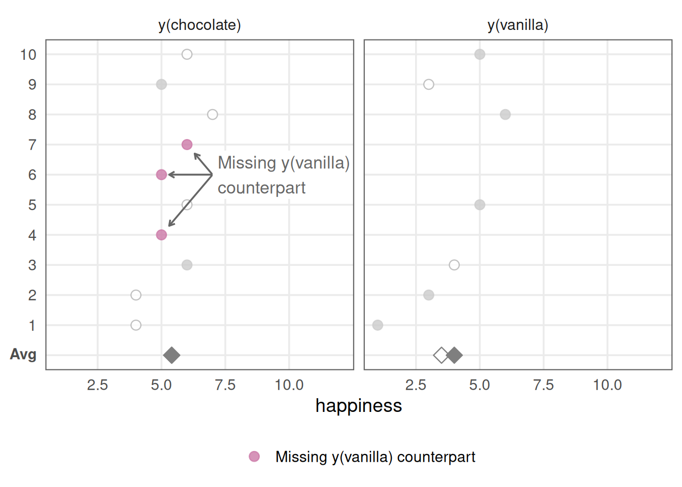

Figure 3.4: 存在结构性正值性违反时的潜在结局。当某个潜在结局不可能发生时，它就没有定义。对香草过敏者不存在对应的 y(vanilla)。

我们可以采取一些措施来改善正值性问题。 对于随机性正值性违反，可以收集更多数据。 增加样本量能够降低随机性违反的概率。 然而，由于要求正值性在每一种协变量组合下成立，我们通常需要使用统计模型，在数据的多维空间中进行外推。 我们将在?sec-ps和?sec-g-comp进一步讨论这一主题。 此外，可以规定入选标准（将在 Section 3.3.2 中讨论），排除那些不可能接受某一暴露水平的人。 如果正值性问题出现在某个特定混杂因素内，也可以考虑移除该混杂因素；若不控制它所导致的混杂偏倚小于正值性问题导致的偏倚，这种权衡可能值得。 最后，我们可以修改试图估计的因果目标估计量。 正如 ?sec-estimands 将展示的，不同因果效应对满足因果假设的严格程度有所不同。

3.2.3 一致性

一致性假设要求，你声称要回答的因果问题与分析实际回答的问题一致。 一致性使我们能够看到每组的一个潜在结局，即事实结局。 在数学上，这意味着 \(Y_{obs} = (X)Y(1) + (1 - X)Y(0)\)。 用通俗语言来说，一致性假设指出，给定处理值下的潜在结局，等于某人被分配该处理值时实际观察到的数值。 这样说来，似乎有些显而易见。 否则还能是什么呢？ 但仔细思考就会发现，对于任何给定暴露，这一假设都很容易被违反。 让我们考虑两种常见情形：

• 定义不清的暴露：对于每个暴露值，实际给予该暴露的方式在受试者之间存在差异。 换言之，存在多个处理版本。 我们需要的是定义明确的暴露。
• 干扰：任何受试者的结局（严格来说，是其所有潜在结局，无论是否被观察到）取决于另一名受试者的暴露；而我们需要的是无干扰。

一致性有时称为稳定单位处理值假设（stable-unit-treatment-value assumption，SUTVA）(Imbens and Rubin 2015)。 不过，因果一致性不同于统计一致性；后者是指随着样本量增加，估计量逐渐接近真实值这一性质。

3.2.3.1 定义不清的暴露

当暴露定义不清时，一致性违反十分常见。 这种问题广泛存在：从手术（例如，一名医生是否比另一名医生更熟悉某项手术操作），到收入（每一美元收入是否都完全相同？ 彩票奖金与每周工资相同吗？）， 再到教育（在学校质量不同时，受教育年限的效应是否相同？），以及其他许多情形 (Rehkopf et al. 2016)。

假设有两盒巧克力冰淇淋，其中一盒已经变质。 “巧克力”暴露可能因个体所取冰淇淋的来源不同而具有不同含义（普通巧克力冰淇淋或变质的巧克力冰淇淋）；但我们把它们全部归在同一个术语下。 无论你通常多么喜欢巧克力冰淇淋，食用变质冰淇淋都会让你痛苦，因此这并不是同一个潜在结局。

data <- tibble(
  id = 1:10,
  y_spoiled_chocolate = c(0, 0, 0, 0, 0, 0, 0, 0, 0, 0),
  y_chocolate = c(4, 4, 6, 5, 6, 5, 6, 7, 5, 6),
  y_vanilla = c(1, 3, 4, 5, 5, 6, 8, 6, 3, 5)
) |>
  mutate(causal_effect = y_chocolate - y_vanilla)

set.seed(11)
data_observed_poorly_defined <- data |>
  mutate(
    exposure_unobserved = case_when(
      rbinom(n(), 1, 0.25) == 1 ~ "chocolate (spoiled)",
      rbinom(n(), 1, 0.25) == 1 ~ "chocolate",
      .default = "vanilla"
    ),
    observed_outcome = recode_values(
      exposure_unobserved,
      "chocolate (spoiled)" ~ y_spoiled_chocolate,
      "chocolate" ~ y_chocolate,
      "vanilla" ~ y_vanilla
    ),
    exposure = recode_values(
      exposure_unobserved,
      c("chocolate (spoiled)", "chocolate") ~ "chocolate",
      "vanilla" ~ "vanilla"
    )
  )

我们知道，样本中（未变质）巧克力的真实平均因果效应为 0.8；然而，估计的因果效应为 -1.9。

data_observed_poorly_defined |>
  group_by(exposure) |>
  summarise(avg_outcome = mean(observed_outcome))

# A tibble: 2 × 2
  exposure  avg_outcome
  <chr>           <dbl>
1 chocolate        2.75
2 vanilla          4.67

我们以为自己正在估计的潜在结局，并不是实际观察到的潜在结局。 我们把新鲜和变质的巧克力冰淇淋视为同一种暴露，但二者对潜在结局的影响不同。 由于暴露是随机的，我们其实相当准确地估计了 y(chocolate, spoiled = FALSE) or y(chocolate, spoiled = TRUE) 的效应，但这不是我们关注的对象。 我们只想得到 y(chocolate, spoiled = FALSE)。

plot_data <- data_observed_poorly_defined |>
  mutate(is_spoiled = exposure_unobserved == "chocolate (spoiled)") |>
  pivot_longer(
    cols = starts_with("y"),
    names_prefix = "y_",
    names_to = "potential_outcome",
    values_to = "happiness"
  ) |>
  filter(
    !(is_spoiled & potential_outcome == "chocolate"),
    !(!is_spoiled & potential_outcome == "spoiled_chocolate")
  ) |>
  mutate(
    potential_outcome = case_when(
      potential_outcome == "spoiled_chocolate" ~ "chocolate",
      TRUE ~ potential_outcome
    ),
    observed = if_else(exposure == potential_outcome, "observed", "unobserved"),
    potential_outcome = paste0("y(", potential_outcome, ")")
  ) |>
  mutate(observed = factor(observed, levels = c("observed", "unobserved"))) |>
  arrange(id) |>
  mutate(y_id = dense_rank(id))

avg_labels <- compute_avg_labels(
  plot_data,
  c("potential_outcome", "exposure", "observed")
)

# Annotations for spoiled chocolate
spoiled_annotation <- plot_data |>
  filter(is_spoiled, potential_outcome == "y(chocolate)") |>
  slice(1) |>
  mutate(label = "Their chocolate was spoiled")

spoiled_arrows <- plot_data |>
  filter(is_spoiled, potential_outcome == "y(chocolate)") |>
  mutate(
    xend = happiness + c(0.35, 0.05),
    yend = y_id - c(0, 0.2),
    x = spoiled_annotation$happiness + 1.9,
    y = spoiled_annotation$y_id + 0.5
  )

flawed_avg_annotation <- avg_labels |>
  filter(
    potential_outcome == "y(chocolate)",
    exposure == "chocolate",
    observed == "observed"
  ) |>
  mutate(
    label = "This is an average of\nboth potential outcomes",
    x = happiness + 2.25,
    y = y_id + 0.9,
    happiness = happiness + 0.25,
    y_id = y_id + 0.15
  )

unspoiled_annotation <- plot_data |>
  filter(
    !is_spoiled,
    exposure == "chocolate",
    potential_outcome == "y(chocolate)",
    observed == "observed"
  ) |>
  slice(1) |>
  mutate(
    label = "But theirs\nwasn't",
    x = happiness + 2,
    y = y_id
  )

unspoiled_arrows <- plot_data |>
  filter(
    !is_spoiled,
    exposure == "chocolate",
    potential_outcome == "y(chocolate)",
    observed == "observed"
  ) |>
  mutate(
    xend = happiness + 0.35,
    yend = y_id - c(0.1, 0.2),
    x = unspoiled_annotation$x,
    y = unspoiled_annotation$y
  )

ggplot(plot_data, aes(x = happiness, y = y_id)) +
  geom_point(
    data = plot_data |> filter(!is_spoiled, observed == "observed"),
    size = 3,
    shape = 21,
    fill = "grey50",
    color = "grey50",
    alpha = 0.8
  ) +
  geom_point(
    data = plot_data |> filter(!is_spoiled, observed == "unobserved"),
    size = 3,
    shape = 21,
    fill = "white",
    color = "grey50",
    alpha = 0.8
  ) +
  geom_point(
    data = plot_data |>
      filter(
        is_spoiled,
        potential_outcome == "y(chocolate)",
        observed == "observed"
      ),
    size = 3,
    shape = 21,
    fill = ggokabeito::palette_okabe_ito(7),
    color = ggokabeito::palette_okabe_ito(7),
    alpha = 0.8
  ) +
  geom_point(
    data = plot_data |>
      filter(
        is_spoiled,
        potential_outcome == "y(chocolate)",
        observed == "unobserved"
      ),
    size = 3,
    shape = 21,
    fill = "white",
    color = ggokabeito::palette_okabe_ito(7),
    alpha = 0.8
  ) +
  add_avg_layers(avg_labels) +
  geom_curve(
    data = spoiled_arrows,
    mapping = aes(x = x, xend = xend, y = y, yend = yend),
    curvature = -0.2,
    arrow = arrow(length = unit(0.02, "npc")),
    inherit.aes = FALSE,
    color = "grey40"
  ) +
  geom_label(
    data = spoiled_annotation,
    mapping = aes(x = happiness + 2, y = y_id + 0.5, label = label),
    hjust = 0,
    inherit.aes = FALSE,
    color = "grey40",
    size = 4,
    linewidth = NA
  ) +
  geom_curve(
    data = flawed_avg_annotation,
    mapping = aes(x = x, xend = happiness, y = y, yend = y_id),
    curvature = 0.2,
    arrow = arrow(length = unit(0.02, "npc")),
    inherit.aes = FALSE,
    color = "grey40"
  ) +
  geom_label(
    data = flawed_avg_annotation,
    mapping = aes(x = x, y = y, label = label),
    hjust = 0,
    inherit.aes = FALSE,
    color = "grey40",
    size = 4,
    linewidth = NA
  ) +
  geom_curve(
    data = unspoiled_arrows,
    mapping = aes(x = x, xend = xend, y = y, yend = yend),
    curvature = -0.2,
    arrow = arrow(length = unit(0.02, "npc")),
    inherit.aes = FALSE,
    color = "grey40"
  ) +
  geom_label(
    data = unspoiled_annotation,
    mapping = aes(x = x, y = y, label = label),
    hjust = 0,
    inherit.aes = FALSE,
    color = "grey40",
    size = 4,
    linewidth = NA
  ) +
  facet_wrap(~potential_outcome) +
  scale_y_continuous(
    breaks = c(unique(plot_data$y_id), min(plot_data$y_id) - 1),
    labels = c(unique(plot_data$id), expression(bold("Avg")))
  ) +
  scale_x_continuous(breaks = seq(0, 12, by = 2.5), limits = c(NA, 12)) +
  labs(y = "actual exposure") +
  po_theme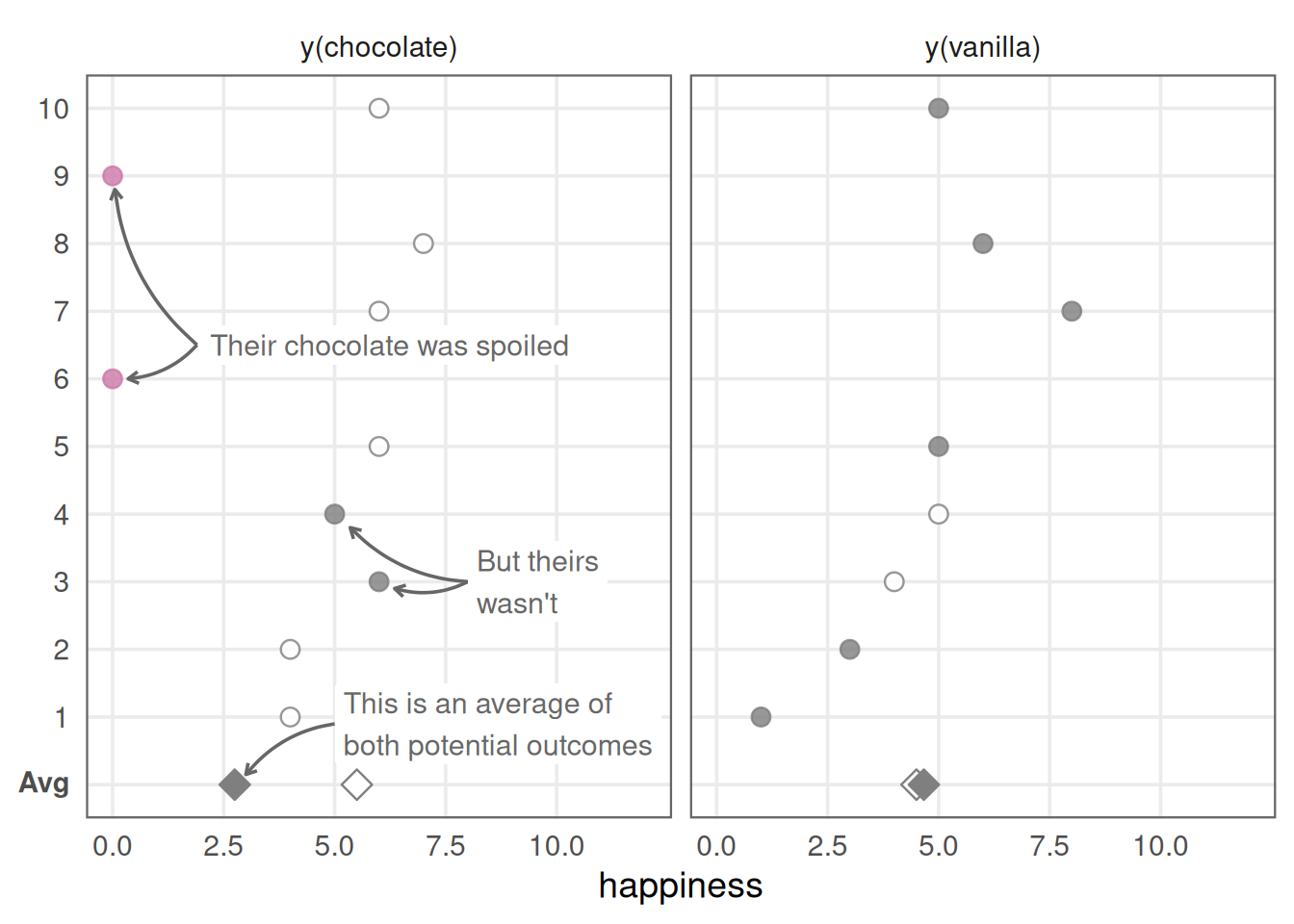

Figure 3.5: 一致性违反下的潜在结局。一致性使我们能够把观察数据视为事实结局。这里，我们把巧克力组视为 y(chocolate) 的代表，但事实并非如此。这些数据混合了 y(chocolate, spoiled = FALSE) 和 y(chocolate, spoiled = TRUE)，而二者是不同的潜在结局。

我们还可以想象处理发生细微变化的其他方式：高质量和低质量品牌的香草冰淇淋都被归类为”香草”。 一个人在早晨食用，另一个人在下午食用。 一个人只吃一勺，另一个人吃满满三碗。 从这个意义上说，几乎总会存在某种一致性违反；我们需要判断的是，这种违反对于所观察的潜在结局是否具有实质意义。 如果两个冰淇淋品牌产生相同的幸福感，这种差异就不重要。 如果不同，差异又有多大？

除更精确地定义暴露外，处理一致性违反的一种方法是调查处理水平内部可能存在的偏离。 假设实验结束后我们检测了冰淇淋容器，并在数据中记录了冰淇淋是否变质。 现在可以按实际暴露进行分组。

data_observed_poorly_defined |>
  group_by(exposure_unobserved) |>
  summarise(avg_outcome = mean(observed_outcome))

# A tibble: 3 × 2
  exposure_unobserved avg_outcome
  <chr>                     <dbl>
1 chocolate                  5.5 
2 chocolate (spoiled)        0   
3 vanilla                    4.67

现在我们重新得到了正确答案，因为在分析中正确地区分了潜在结局，如 Figure 3.6 所示。

plot_data <- data_observed_poorly_defined |>
  pivot_longer(
    cols = starts_with("y"),
    names_prefix = "y_",
    names_to = "potential_outcome",
    values_to = "happiness"
  ) |>
  mutate(
    potential_outcome = if_else(
      potential_outcome == "spoiled_chocolate",
      "chocolate (spoiled)",
      potential_outcome
    ),
    observed = if_else(
      exposure_unobserved == potential_outcome,
      "observed",
      "unobserved"
    ),
    potential_outcome = if_else(
      potential_outcome == "chocolate (spoiled)",
      "spoiled_chocolate",
      potential_outcome
    ),
    potential_outcome = paste0("y(", potential_outcome, ")")
  ) |>
  arrange(id) |>
  mutate(y_id = dense_rank(id))

avg_labels <- compute_avg_labels(
  plot_data,
  c("potential_outcome", "exposure_unobserved", "observed")
)

ggplot(plot_data, aes(x = happiness, y = y_id, color = exposure_unobserved)) +
  geom_point(
    data = plot_data |> filter(observed == "observed"),
    mapping = aes(fill = exposure_unobserved),
    size = 3,
    shape = 21,
    alpha = 0.8
  ) +
  geom_point(
    data = plot_data |> filter(observed == "unobserved"),
    size = 3,
    shape = 21,
    fill = "white",
    alpha = 0.8
  ) +
  geom_point(
    data = avg_labels |> filter(observed == "unobserved"),
    aes(x = happiness, y = y_id, color = exposure_unobserved),
    size = 4,
    shape = 23,
    fill = "white",
    inherit.aes = FALSE
  ) +
  geom_point(
    data = avg_labels |> filter(observed == "observed"),
    aes(
      x = happiness,
      y = y_id,
      fill = exposure_unobserved,
      color = exposure_unobserved
    ),
    size = 4,
    shape = 23,
    inherit.aes = FALSE
  ) +
  facet_wrap(~potential_outcome) +
  scale_y_continuous(
    breaks = c(unique(plot_data$y_id), min(plot_data$y_id) - 1),
    labels = c(unique(plot_data$id), expression(bold("Avg")))
  ) +
  scale_fill_manual(values = ggokabeito::palette_okabe_ito(c(1, 2, 7))) +
  scale_color_manual(values = ggokabeito::palette_okabe_ito(c(1, 2, 7))) +
  scale_x_continuous(breaks = seq(0, 12, by = 2.5), limits = c(NA, 12)) +
  labs(
    y = "True exposure",
    color = NULL,
    fill = NULL
  ) +
  po_theme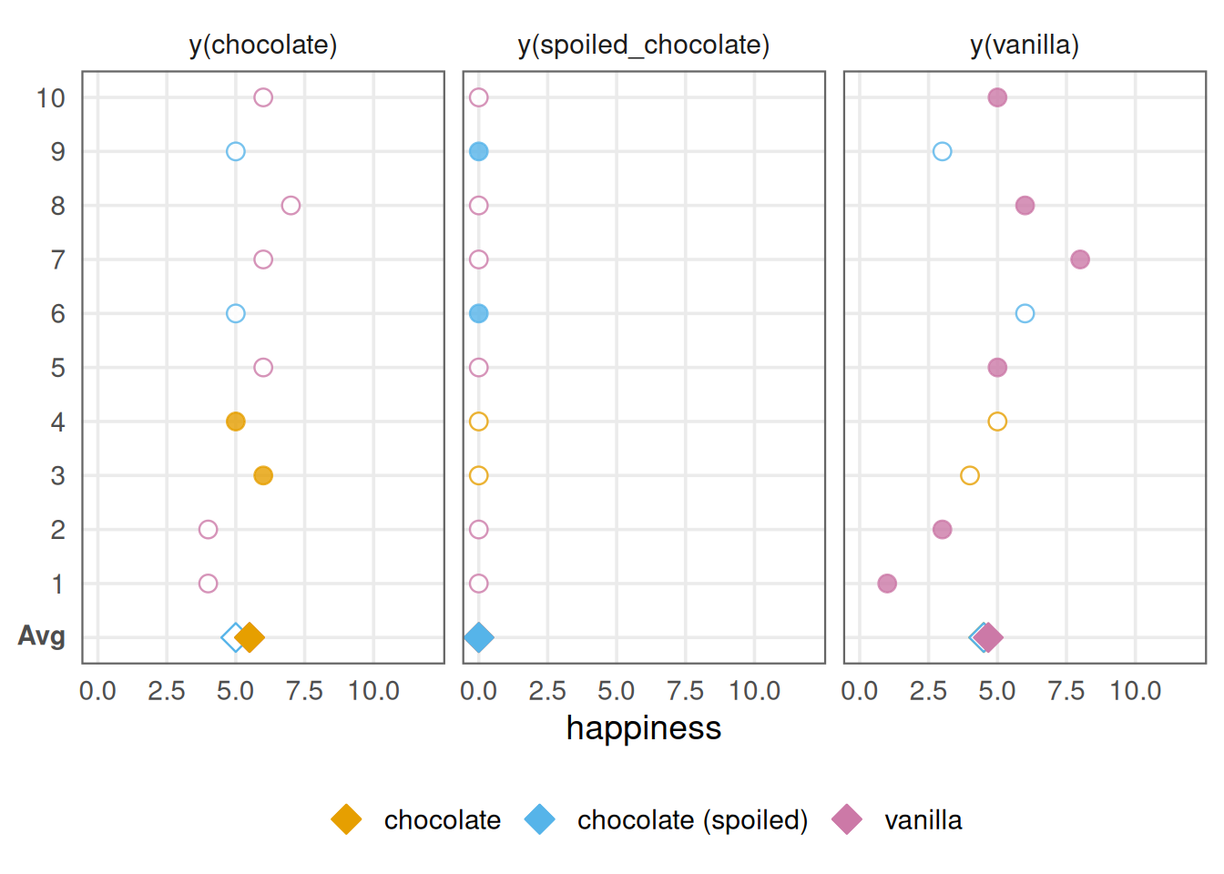

Figure 3.6: 一致性违反下的潜在结局。现在，我们已将观察数据与其底层潜在结局正确关联，从而使二者保持一致。

3.2.3.2 干扰

干扰意味着一名个体的暴露会影响另一名个体的潜在结局。 这种现象在传染病中十分常见，因为某人接种疫苗或接受治疗往往会影响其他人的结局风险。 不过，干扰也可能出现在许多其他情境中，包括通过社交网络、政策干预、接受处理单位之间的地理邻近性等途径发生。

假设冰淇淋研究中的每名个体都有一名搭档，其潜在结局既取决于自己食用的冰淇淋口味，也取决于搭档食用的口味。 在下面的模拟中，若搭档食用不同口味的冰淇淋，个体幸福感会增加两个单位。

data <- tibble(
  id = 1:10,
  partner_id = c(1, 1, 2, 2, 3, 3, 4, 4, 5, 5),
  y_chocolate_chocolate = c(4, 4, 6, 5, 6, 5, 6, 7, 5, 6),
  y_vanilla_vanilla = c(1, 3, 4, 5, 5, 6, 8, 6, 3, 5)
) |>
  # partner's happiness increases by 2
  # when they get a different flavor
  mutate(
    y_chocolate_vanilla = y_chocolate_chocolate + 2,
    y_vanilla_chocolate = y_vanilla_vanilla + 2
  )

set.seed(37)
data_observed_interf <- data |>
  mutate(
    exposure = if_else(
      rbinom(n(), 1, 0.5) == 1,
      "chocolate",
      "vanilla"
    ),
    exposure_partner = if_else(
      rbinom(n(), 1, 0.5) == 1,
      "chocolate",
      "vanilla"
    ),
    observed_outcome = case_when(
      exposure == "chocolate" & exposure_partner == "chocolate" ~
        y_chocolate_chocolate,
      exposure == "chocolate" & exposure_partner == "vanilla" ~
        y_chocolate_vanilla,
      exposure == "vanilla" & exposure_partner == "chocolate" ~
        y_vanilla_chocolate,
      exposure == "vanilla" & exposure_partner == "vanilla" ~
        y_vanilla_vanilla
    )
  )

与暴露定义不清的情况一样，存在干扰时我们无法得到正确答案。

data_observed_interf |>
  group_by(exposure) |>
  summarise(avg_outcome = mean(observed_outcome))

# A tibble: 2 × 2
  exposure  avg_outcome
  <chr>           <dbl>
1 chocolate        6.25
2 vanilla          6.33

同样，问题在于我们估计了错误的潜在结局（Figure 3.7）。 干扰和定义不清的暴露，是违反同一假设的不同表现。 我们所估计的潜在结局与提出的因果问题并不一致。 在本例中存在三个反事实：个体实际食用的口味与搭档未食用口味的组合，以及个体未食用的口味与搭档可能食用的两种口味的组合。 我们计算的平均值似乎没有估计这些组合中的任何一个。

plot_data <- data_observed_interf |>
  pivot_longer(
    cols = starts_with("y_"),
    names_prefix = "y_",
    names_to = "po_combination",
    values_to = "happiness"
  ) |>
  mutate(
    potential_outcome = paste0("y(", str_remove(po_combination, "_.*"), ")"),
    observed = po_combination == paste0(exposure, "_", exposure_partner),
    flavor_match = if_else(
      exposure == exposure_partner,
      "Same Flavors",
      "Different Flavors"
    ),
    y_id = dense_rank(id)
  ) |>
  filter(
    observed | (potential_outcome != exposure)
  )

# Select two observed points for different flavor matches (Chocolate panel)
flavor_annotation <- plot_data |>
  filter(observed, potential_outcome == "y(chocolate)", id %in% c(3, 5)) |>
  summarize(
    x = max(happiness) + 0.5,
    y = mean(y_id) - 2,
    label = str_wrap(
      "Different exposure pairs yield different potential outcomes",
      20
    ),
    potential_outcome = "y(chocolate)"
  )

# Generate arrows for the flavor difference annotation
flavor_arrows <- plot_data |>
  filter(observed, potential_outcome == "y(chocolate)", id %in% c(3, 5)) |>
  mutate(
    xend = happiness,
    yend = y_id - 0.3,
    x = flavor_annotation$x,
    y = flavor_annotation$y,
    potential_outcome = "y(chocolate)"
  )

# Select a single ID with two unobserved potential outcomes (Vanilla panel)
unobserved_id <- 5

unobserved_annotation <- plot_data |>
  filter(!observed, id == unobserved_id, potential_outcome == "y(vanilla)") |>
  summarize(
    x = max(happiness) + 0.75,
    y = mean(y_id) - 0.5,
    label = str_wrap(
      "There are two unobserved potential outcomes for the opposite exposure",
      20
    ),
    potential_outcome = "y(vanilla)"
  )

# Generate arrows for the unobserved potential outcomes for the selected ID
unobserved_arrows <- plot_data |>
  filter(!observed, id == unobserved_id, potential_outcome == "y(vanilla)") |>
  mutate(
    xend = happiness + c(0.35, 0.15),
    yend = y_id - c(0.1, 0.2),
    x = unobserved_annotation$x,
    y = unobserved_annotation$y,
    potential_outcome = "y(vanilla)"
  )

# Select ID 6's unobserved chocolate potential outcome annotation (Chocolate panel)
chocolate_unobserved_annotation <- plot_data |>
  filter(id == 6, potential_outcome == "y(chocolate)", !observed) |>
  summarize(
    x = min(happiness) - 2.5,
    y = mean(y_id) + 0.75,
    label = str_wrap(
      "There is an unobserved potential outcome for the partner's other flavor",
      15
    ),
    potential_outcome = "y(chocolate)"
  )

# Generate arrow pointing to the unobserved chocolate potential outcome for ID 6
chocolate_unobserved_arrow <- plot_data |>
  filter(id == 6, potential_outcome == "y(chocolate)", !observed) |>
  mutate(
    xend = happiness - 0.25,
    yend = y_id + 0.1,
    x = chocolate_unobserved_annotation$x,
    y = chocolate_unobserved_annotation$y,
    potential_outcome = "y(chocolate)"
  )

# Create Plot 5
ggplot(plot_data, aes(x = happiness, y = y_id)) +
  geom_point(
    data = plot_data |> filter(observed),
    mapping = aes(fill = flavor_match, color = flavor_match),
    size = 3,
    shape = 21,
    alpha = 0.8
  ) +
  geom_point(
    data = plot_data |> filter(!observed),
    size = 3,
    shape = 21,
    fill = "white",
    color = "grey70",
    alpha = 0.8
  ) +
  geom_curve(
    data = flavor_arrows,
    mapping = aes(x = x, xend = xend, y = y, yend = yend),
    curvature = -0.2,
    arrow = arrow(length = unit(0.02, "npc")),
    inherit.aes = FALSE,
    color = "grey40"
  ) +
  geom_label(
    data = flavor_annotation,
    mapping = aes(x = x, y = y, label = label),
    hjust = 0,
    inherit.aes = FALSE,
    color = "grey40",
    size = 3,
    linewidth = NA
  ) +
  geom_curve(
    data = unobserved_arrows,
    mapping = aes(x = x, xend = xend, y = y, yend = yend),
    curvature = -0.2,
    arrow = arrow(length = unit(0.02, "npc")),
    inherit.aes = FALSE,
    color = "grey40"
  ) +
  geom_label(
    data = unobserved_annotation,
    mapping = aes(x = x, y = y, label = label),
    hjust = 0,
    inherit.aes = FALSE,
    color = "grey40",
    size = 3,
    linewidth = NA
  ) +
  geom_curve(
    data = chocolate_unobserved_arrow,
    mapping = aes(x = x, xend = xend, y = y, yend = yend),
    curvature = -0.2,
    arrow = arrow(length = unit(0.02, "npc")),
    inherit.aes = FALSE,
    color = "grey40"
  ) +
  geom_label(
    data = chocolate_unobserved_annotation,
    mapping = aes(x = x, y = y, label = label),
    hjust = 1,
    inherit.aes = FALSE,
    color = "grey40",
    size = 3,
    linewidth = NA
  ) +
  facet_wrap(~potential_outcome) +
  scale_y_continuous(
    breaks = unique(plot_data$y_id),
    labels = unique(plot_data$id)
  ) +
  scale_fill_manual(
    values = c(
      "Same Flavors" = ggokabeito::palette_okabe_ito(3),
      "Different Flavors" = ggokabeito::palette_okabe_ito(5)
    ),
    name = NULL
  ) +
  scale_color_manual(
    values = c(
      "Same Flavors" = ggokabeito::palette_okabe_ito(3),
      "Different Flavors" = ggokabeito::palette_okabe_ito(5)
    ),
    name = NULL
  ) +
  scale_x_continuous(breaks = seq(0, 12, by = 2.5), limits = c(NA, 12)) +
  labs(
    x = "Happiness",
    y = "ID"
  ) +
  po_theme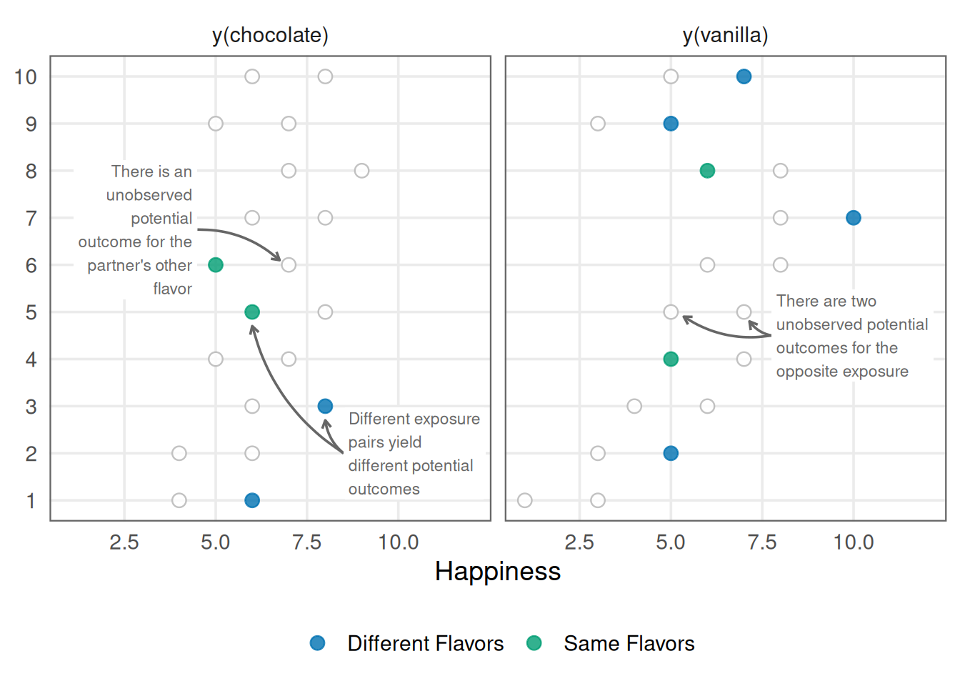

Figure 3.7: 一致性违反下的潜在结局。这一次，香草组的 y(vanilla) 和巧克力组的 y(chocolate) 并不正确：它们混合了搭档口味所产生的干扰效应。

与之前一样，我们可以更明确地定义潜在结局。

data_observed_interf |>
  group_by(exposure, exposure_partner) |>
  summarise(avg_outcome = mean(observed_outcome), .groups = "drop")

# A tibble: 4 × 3
  exposure  exposure_partner avg_outcome
  <chr>     <chr>                  <dbl>
1 chocolate chocolate               5.5 
2 chocolate vanilla                 7   
3 vanilla   chocolate               6.75
4 vanilla   vanilla                 5.5 

应对干扰的主要方法之一，是改变所考虑的单位。 这里，每名个体、每个唯一 ID 都被视为一个单位，而单位之间（即搭档之间）存在干扰。 假设我们把每一对搭档视为一个单位，并对搭档组合而非个体进行随机化。 这样便能解决干扰问题，因为不同搭档组合之间不存在干扰。 这种随机化有时称为整群随机试验。 每个群组内部如何处理，可能取决于当前的因果问题。 例如，若想知道两个人都食用巧克力冰淇淋与都食用香草冰淇淋相比会发生什么，就应将一对搭档随机分配为都食用巧克力或都食用香草，如下所示。

set.seed(11)

## we are now randomizing the *partnerships* not the individuals
partners <- tibble(
  partner_id = 1:5,
  exposure = if_else(
    rbinom(5, 1, 0.5) == 1,
    "chocolate",
    "vanilla"
  )
)
partners_observed <- data |>
  left_join(partners, by = "partner_id") |>
  mutate(
    # all partnerships have the same exposure
    exposure_partner = exposure,
    observed_outcome = case_when(
      exposure == "chocolate" & exposure_partner == "chocolate" ~
        y_chocolate_chocolate,
      exposure == "vanilla" & exposure_partner == "vanilla" ~
        y_vanilla_vanilla
    )
  )

现在，我们可以检测到正确的因果效应。

partners_observed |>
  group_by(exposure) |>
  summarise(avg_outcome = mean(observed_outcome))

# A tibble: 2 × 2
  exposure  avg_outcome
  <chr>           <dbl>
1 chocolate        5.5 
2 vanilla          4.38

也有一些方法可在存在多个处理版本或干扰时识别效应，但这些方法技术性较强，并且在相应一致性违反下受到更多限制 (Tchetgen and VanderWeele 2010; VanderWeele and Hernan 2013)。

类似地，可以为搭档分配相同或不同口味，从而计算跨口味效应。 另一种选择是排除有搭档者，使干扰效应不再存在。 关键是思考希望估计什么，并尽可能精确地表示该问题对应的潜在结局。

Note再谈疟疾蚊帐

在 Chapter 2 中，我们估计了蚊帐对疟疾风险的因果效应。 下面考虑该问题的因果假设，以及它们在现实分析中可能如何被违反。

• 可交换性：我们已经看到，当存在未测量混杂因素（本例中为遗传性疟疾抗性）时，这个问题会产生怎样的后果。 在使用观察数据进行因果推断时，思考可交换性是要求较高且十分常见的任务之一。 我们将在 Chapter 4 中深入讨论这一点，并在 ?sec-sensitivity 中讨论当我们认为（或知道）自己错了时该怎么办。 我们还应担心所需协变量是否测量得不够准确，或者是否存在缺失值（?sec-missingness）。
• 正值性：如果任何家庭始终使用或从不使用蚊帐，就会违反正值性。 现实中完全可能出现这种情况。 有人可能对蚊帐材料过敏，或者某种蚊帐可能未获某个地区批准。 如前所述，正值性还需要在分析所用混杂因素组合的各水平内成立。 例如，经济状况较差、生活在寒冷天气中（此时蚊虫不太活跃）且健康状况良好的人，是否可能因为认为不值得花钱而从不使用蚊帐？
• 一致性：我们已经见过暴露定义明确性问题的一个例子：“蚊帐”可能具有许多不同含义。 我们决定比较经杀虫剂处理的蚊帐与不使用蚊帐，但可能还需要更具体。 制造商是否重要？ 杀虫剂类型呢？ 杀虫剂用量呢？ 我们需要思考这些变化分别可能对潜在结局产生怎样的影响。 干扰是蚊帐研究中的真实问题，尤其对于杀虫蚊帐而言。 值得注意的是，我们使用家庭作为观察单位，这会减少部分局部干扰。 还可以考虑彼此地理位置分散的家庭。

3.3 研究设计何时支持因果推断？

可交换性、正值性和一致性都是简单的假设，但正如我们所见，它们很容易被违反。 当某种因果方法的假设不成立时，我们就无法用观察数据模拟反事实，并将其与观察结局进行比较。 不过，无论是在收集数据之前，还是在处理”现成的”观察数据时，都可以通过周密的研究设计应对许多潜在的假设违反。

3.3.1 随机试验

正如我们所见，随机试验在满足所需因果假设方面具有优良性质。 在极限意义下，我们预期可交换性成立，因为暴露的唯一原因是随机化过程本身。 由于随机化过程是随机的，它与研究中的潜在结局完全独立。 类似地，只要没有人的暴露是确定性的，随机化过程就能保证正值性；因为用于分配暴露的概率是已知的。 随机试验也有助于满足一致性，尤其有助于使暴露定义明确，但并不能保证一致性。 只有先定义暴露，才能实施暴露。 不过，干扰仍可能发生。 例如，如果将一些人随机分配为接种传染病疫苗，他们接种疫苗可能会改变周围人的暴露概率，从而降低周围人感染的可能性。 这就要求在试验设计中作额外考虑，例如像上述示例那样采用整群随机化或分隔研究单位。

我们将暴露被随机分配的分析称为随机试验。 这种随机化设计有时称为 A/B 测试，意即”A 和 B 哪个更好？” A/B 测试在业界很常见，例如用于测试两种不同的网站用户界面设计。 但从本质上说，它们都是随机实验，因此本节的所有内容仍然适用。

然而，这些性质属于理想的随机试验。 在真实的随机试验中，可能会出现问题。 样本量过小时，可交换性可能偶然失效。 人们也不一定会按要求行事；研究中的许多人不会依从所分配的暴露。 不依从的原因往往会造成可交换性问题。 类似地，研究对象可能以导致不可交换性的方式退出研究。 我们将在 ?sec-longitudinal 和 ?sec-iv-friends 中更深入地讨论这些主题及其应对方法。 真实试验中的暴露也可能不一致，原因可能来自实施者（如上述手术示例），也可能来自参与者。 例如，参与者可能被要求每天服用两片药，却决定每天只服用一片。 防止干扰的尝试也可能失败，例如对错误的单位进行随机化，或不同单位以意外方式相互作用。

非随机化研究（观察性研究）即使处于理想状态，也没有这些保证。 与现实随机试验一样，观察性研究需要精心设计和实施，才能更好地满足因果推断所需的假设。 Table 3.4 总结了理想随机试验、现实随机试验和观察性研究分别在多大程度上满足可交换性、正值性和一致性标准。

假设	理想随机试验	现实随机试验	观察性研究
一致性（暴露定义明确）	😄	🤷	🤷
一致性（无干扰）	🤷	🤷	🤷
正值性	😄	😄	🤷
可交换性	😄	🤷	🤷

Table 3.4: 通过研究设计解决的假设。 😄 表示默认已解决，r emo::ji("shrug") 表示该问题可以解决，但默认并未解决。

因果分析的设计需要一个清晰的因果问题。 随后可以将该问题映射到一份研究方案；按照 Hernán and Robins (2016) 的定义，该方案由构成目标试验框架的以下七个要素组成：

• 入选标准：应将哪些人或事物纳入研究？
• 暴露定义：符合资格后，研究单位将接受何种明确的暴露？
• 分配程序：如何将符合资格的单位分配至某项暴露？
• 随访期：随访何时开始、何时结束？
• 结局定义：将测量哪些明确的结局？
• 关注的因果对比：将估计哪个因果目标估计量？
• 分析计划：将对数据实施哪些数据处理和统计程序，以估计关注的因果对比？

回顾 Section 1.3 中的图 (Figure 1.6)； 在尝试定义因果问题时，可以将其中若干研究方案要素映射到这些图中。

Figure 3.8: 映射到因果分析术语的示例图

3.3.2 模拟目标试验

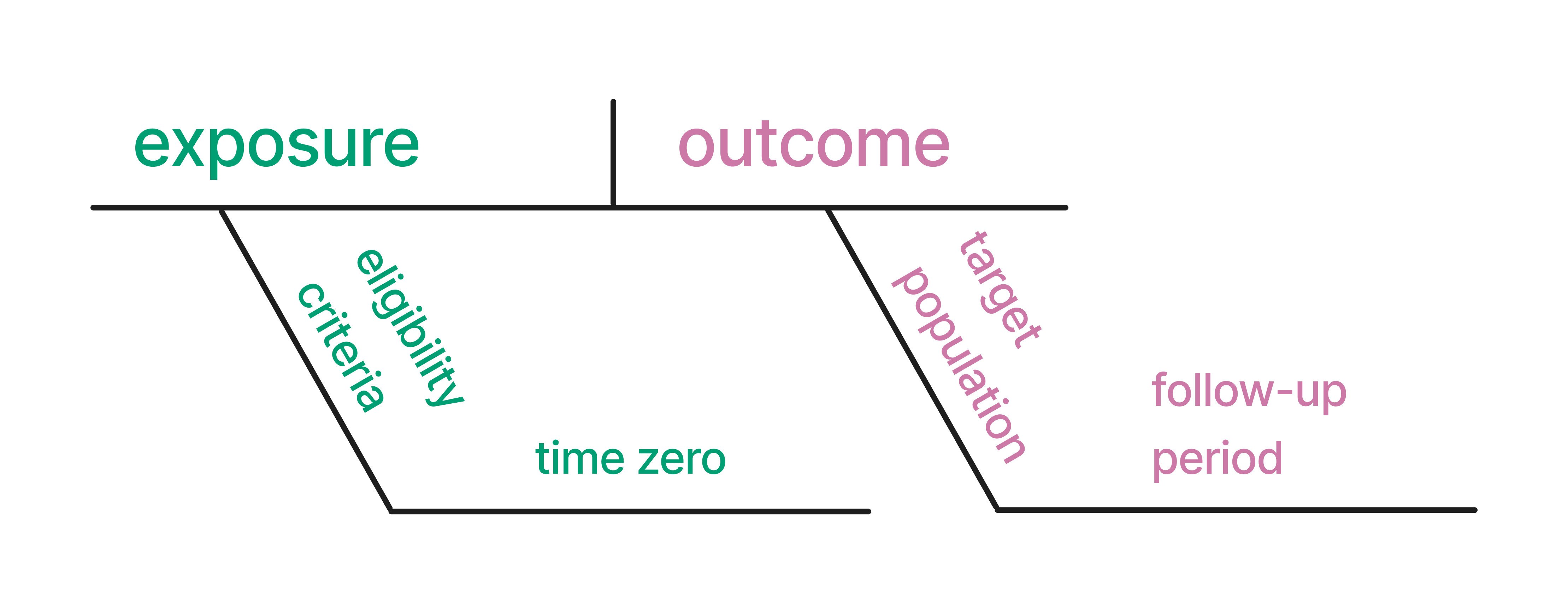
随机试验有助于满足因果假设，但如 Chapter 1 所述，由于时间、资金和伦理等多种原因，我们可能无法实施随机化。 在随机试验开展期间，我们也可能利用观察数据更早获得初步答案。

即使不开展随机试验，设想这类试验将如何进行，也能提高基于观察数据所得推断的质量。 这就是目标试验模拟背后的思想：先明确一个目标试验（你会开展或过去已经开展的随机试验），再尝试使用观察数据模拟该设计。

无论采用随机试验还是观察性研究设计，使用研究方案都能提高满足因果假设的可能性。 在 Table 3.5 中，我们将这些要素映射到它们可以处理的相应假设。

假设	入选标准	暴露定义	分配程序	随访期	结局定义	因果对比	分析计划
一致性（暴露定义明确）	✔️	✔️	✔️				✔️
一致性（无干扰）	✔️	✔️	✔️		✔️		✔️
正值性	✔️	✔️	✔️			✔️	✔️
可交换性	✔️	✔️	✔️	✔️	✔️	✔️	✔️

Table 3.5: 将假设映射到研究方案要素

• 入选标准：入选标准有助于防止违反正值性（排除那些绝不可能接受某项暴露的人），同时也有助于满足一致性和可交换性。 例如，可以排除可能影响彼此结局的人，或只纳入不具有极端特征的人。
• 暴露定义：精确的暴露定义对改善一致性尤其有用，因为它促使暴露定义明确，并能更好地控制潜在干扰。 精确的暴露也有助于识别与可交换性和正值性相关的因素。
• 分配程序：随机分配能够满足可交换性和正值性。 了解暴露如何发生，也能改善非随机化研究中的可交换性和正值性。 正如我们所见，分配程序还可以用于防止干扰；同样，由于分配机制需要精确，它也有助于使暴露定义更加明确。
• 随访期：我们将在 ?sec-longitudinal 中更详细地讨论定义随访期所解决的问题；它通过确保各暴露水平的随访时间具有可比性，帮助满足可交换性。 它也与一致性密切相关，因为定义明确的暴露可能需要包含时间要素。
• 结局定义：精确定义结局有助于识别预后因素，既能提高随机试验的精确性，也能改善观察性研究的可交换性。
• 关注的因果对比：正如 ?sec-estimands 将展示的，某些因果对比对可交换性和正值性的要求没有其他对比那么严格。
• 分析计划：清晰的分析计划能够全面改善观察性研究对因果假设的满足程度。 例如，我们必须明确需要调整哪些变量才能满足可交换性。 此外，尽管永远无法确认某种因果方法的假设确实成立，但可以通过探索性分析 (?sec-data-causal) 提供证据，或通过敏感性分析 (?sec-sensitivity) 探查违反假设的后果。

冰淇淋示例的目标试验及其模拟会是什么样？ 假设我们拥有一个包含全部所需信息的数据库。 一家商店精确供应 100 g 巧克力或香草冰淇淋，两种口味均来自同一品牌。 借助该数据库，我们获得了参与者的口味选择和其他多种特征，包括幸福感（使用与上述相同的工具测量）；幸福感在进店时测量一次（基线），食用冰淇淋 30 分钟后再测量一次（随访）。 在 Table 3.6 中，我们概述了针对该问题开展随机试验的一些设想，以及使用这一数据库模拟该试验的观察性研究。 值得注意的是，我们能够模拟的目标试验通常是所谓的实用性试验—即不设盲的试验。 这是因为通常无法对参与者本人隐藏其所接受的暴露。

研究方案步骤	描述	目标试验	模拟研究
入选标准	应将哪些人纳入研究？	纳入：年龄 18–65 岁。排除：乳糖不耐受或对任何成分过敏；未在研究所在周进入商店。	与目标试验相同。
暴露定义	符合资格后，研究单位将接受何种明确的暴露？	碗装 100 g 香草或巧克力冰淇淋，两者均为 Don and Jerzy 品牌。	与目标试验相同。
分配程序	如何将符合资格的单位分配至某项暴露？	参与者以 50% 的概率随机接受任一口味。分配不设盲。	按照数据所示为参与者分配口味，例如其实际选择的口味。使用基线协变量模拟随机化。
随访期	随访何时开始、何时结束？	开始：满足入选标准并分配口味时；结束：口味分配后 30 分钟。	与目标试验相同。
结局定义	将测量哪些明确的结局？	使用金标准工具测量的幸福感（1–10）。	与目标试验相同。
关注的因果对比	将估计哪个因果目标估计量？	平均处理效应（ATE）。	与目标试验相同。
分析计划	将对数据实施哪些数据处理和统计程序，以估计关注的因果对比？	使用逆概率加权计算 ATE，按基线幸福感、年龄、收入、教育、身体活动、自评身体健康、自评心理健康、关系质量和口味偏好进行加权。	使用逆概率加权计算 ATE，按混杂因素（基线幸福感、年龄、口味偏好）以及其他基线预后变量（年龄、收入、教育、身体活动、自评身体健康、自评心理健康和关系质量）进行加权。

Table 3.6: 冰淇淋口味对幸福感影响的目标试验方案，以及模拟该目标试验的相应观察性研究方案

Table 3.6 中的研究方案以多种方式帮助我们满足因果假设。 例如，排除过敏或敏感人群后，正值性更有可能成立。 当暴露定义明确时，一致性也更有可能成立。 如果认为干扰是一个问题，还可以改变随机化程序，采用整群设计，或排除我们认为可能相互干扰的人（例如，每组只纳入一人）。 我们还尝试通过 IPW 复现随机化，以处理可交换性。 对于这个因果问题，我们认为口味选择和幸福感的共同原因是基线幸福感、年龄和口味偏好。 我们认为幸福感的其他原因包括年龄、收入、教育、身体活动、自评身体健康、自评心理健康和关系质量。 我们将在 Chapter 4 中更详细地讨论这一思想。 这里还有几个要素将在后文进一步讨论。 如前所述，我们将在 ?sec-longitudinal 中讨论随访，在 ?sec-estimands 中讨论目标估计量，包括随机试验特有的目标估计量。 尽管目标试验采用随机化，我们仍然使用 IPW。 我们将在 ?sec-ci-rct 中讨论这样做的益处。

Century, D. 2022. Split Decision: Life Stories. Gallery Books. https://books.google.com/books?id=bN9IEAAAQBAJ.

Hernán, Miguel A, and James M Robins. 2016. “Using Big Data to Emulate a Target Trial When a Randomized Trial Is Not Available.” American Journal of Epidemiology 183 (8): 758–64.

Imbens, Guido W, and Donald B Rubin. 2015. Causal Inference in Statistics, Social, and Biomedical Sciences. Cambridge University Press.

Rehkopf, David H., M. Maria Glymour, and Theresa L. Osypuk. 2016. “The Consistency Assumption for Causal Inference in Social Epidemiology: When a Rose Is Not a Rose.” Current Epidemiology Reports 3 (1): 63–71. https://doi.org/10.1007/s40471-016-0069-5.

Tchetgen, Eric J Tchetgen, and Tyler J VanderWeele. 2010. “On Causal Inference in the Presence of Interference.” Statistical Methods in Medical Research 21 (1): 55–75. https://doi.org/10.1177/0962280210386779.

VanderWeele, Tyler J., and Miguel A. Hernan. 2013. “Causal Inference Under Multiple Versions of Treatment.” Journal of Causal Inference 1 (1): 1–20. https://doi.org/10.1515/jci-2012-0002.

---

1. 根据研究方案，禁止将两种冰淇淋混合食用。

2. 这些因果假设独立于所用估计量要求的任何统计假设，例如分布假设。

3. 由于样本量的原因，数值略有不同。 随着样本量增加，随机化下的可交换性更有可能成立；因此，当样本足够大时，我们会得到相同的答案。